File:Standard Normal Distribution.png
From KYNNpedia

Size of this preview: 800 × 494 pixels. Other resolutions: 320 × 198 pixels | 640 × 396 pixels | 1,024 × 633 pixels | 1,280 × 791 pixels | 2,560 × 1,582 pixels | 5,986 × 3,700 pixels.
Original file (5,986 × 3,700 pixels, file size: 752 KB, MIME type: image/png)
Summary
| Description |
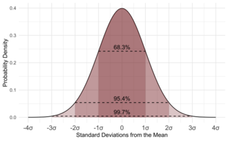
English: The Standard Normal Probability Distribution with shaded regions
Русский: Кривая плотности вероятности нормального распределения с закрашенными областями |
| Date | |
| Source | Own work |
| Author | D Wells |
| Other versions |
[]
|


|
File:Standard Normal Distribution-en.svg is a vector version of this file. It should be used in place of this PNG file when not inferior.
File:Standard Normal Distribution.png → File:Standard Normal Distribution-en.svg
For more information, see Help:SVG. |
 |
<code><code><code><languages/></code></code></code>
Licensing
I, the copyright holder of this work, hereby publish it under the following license:
This file is licensed under the Creative Commons Attribution-Share Alike 4.0 International license.
- You are free:
- to share – to copy, distribute and transmit the work
- to remix – to adapt the work
- Under the following conditions:
- attribution – You must give appropriate credit, provide a link to the license, and indicate if changes were made. You may do so in any reasonable manner, but not in any way that suggests the licensor endorses you or your use.
- share alike – If you remix, transform, or build upon the material, you must distribute your contributions under the same or compatible license as the original.
Source code
library(ggplot2)
p <- ggplot(NULL, aes(c(-4,4))) +
  geom_line(stat = "function", fun = dnorm) +
  geom_area(stat = "function", fun = dnorm, fill = scales::muted("blue"), xlim=c(-1,1), alpha=1/4) +
  geom_area(stat = "function", fun = dnorm, fill = scales::muted("blue"), xlim=c(-2,2), alpha=1/4) +
  geom_area(stat = "function", fun = dnorm, fill = scales::muted("blue"), xlim=c(-3,3), alpha=1/4) +
  theme_minimal() +
  theme(axis.text.x = element_text(size = 12)) +
  scale_x_continuous(labels = label_units, breaks = -4:4) +
  xlab("Standard Deviations from the Mean") +
  ylab("Probability Density") +
  geom_segment(aes(x=-1, xend=1, y=dnorm(1), yend=dnorm(1)), linetype="dashed") +
  geom_segment(aes(x=-2, xend=2, y=dnorm(2), yend=dnorm(2)), linetype="dashed") +
  geom_segment(aes(x=-3, xend=3, y=dnorm(3), yend=dnorm(3)), linetype="dashed") +
  annotate("text", x = 0, y = dnorm(1)+0.015, label = "68.3%") + #pnorm(1)-pnorm(-1) %
  annotate("text", x = 0, y = dnorm(2)+0.015, label = "95.4%") +
  annotate("text", x = 0, y = dnorm(3)+0.015, label = "99.7%")

ggsave("Normal_Distribution.png", p, width = 3.7*1.618, height = 3.7, dpi = 1000)
File history
Click on a date/time to view the file as it appeared at that time.
| Date/Time | Thumbnail | Dimensions | User | Comment | |
|---|---|---|---|---|---|
| current | 18:25, 24 June 2019 | | 5,986 × 3,700 (752 KB) | wikimediacommons>D Wells | User created page with UploadWizard |
File usage
The following page uses this file: